Methodology for estimating the range of a salvo shot point

In the photo from the Forensic Legal Newspaper, the owners turned bullet holes in the fence into flowers.

Methodology for estimating the range of a salvo shot point
based on the actual dispersion of projectiles

During armed conflicts, the parties often accuse each other of shelling peaceful areas, for example, residential areas of cities remote from military installations. Such actions are classified as war crimes and are regulated by international humanitarian law. Both sides can use such attacks for their own propaganda purposes. 

Therefore, establishing the truth in such cases is critical. To answer the question of who carried out the shelling, you need to know two indicators of the point of the shot: 1) its azimuth and 2) range. 

In the case of an unguided projectile, the azimuth of the shot point can be quite accurately determined by the shape and characteristic elements of the crater from its impact [1], by the position of the remainder of the projectile stuck in the obstacle, and by a number of other additional features. 

As a rule, the situation with estimating the range of the shot point is much more complicated. In the case of a single shot, the only way to make such an assessment is to analyze the angle of inclination of the remainder of the projectile stuck in the obstacle. However, firstly, such a possibility is not always possible, and secondly, this method can produce a significant error due to a large number of random and uncertain factors. 

During salvo fire, for example, from a multiple launch rocket system (MLRS), it is possible to estimate the range of the firing point by the dispersion of projectiles [2]. The methodology for such an assessment is presented below.

From the theory and practice of artillery shooting it is known that during a salvo shot, the dispersion of projectile impact points obeys the normal distribution law, resulting in the formation of a so-called “dispersion ellipse” [2; 3, p. 19; 4, p. 217]. The dimensions of this ellipse in artillery are usually characterized by the values ​​of the median deviations along the range B d and along the front (width) B b. In Fig. Figure 1 shows the probability of falling into the cells of the scattering ellipse, multiples of the median deviations B d and B b (more precisely, into the cells of the rectangle described around this ellipse). For example, the probability of getting into a small central square of four cells from D4 to E5 (we will denote the cell interval as D4:E5) is 25%.

To determine the most probable range from which the shot was fired, a method of mathematical statistics is used, which is widely used for estimating an unknown parameter - the maximum likelihood method . The essence of the method is that the desired value of the parameter is estimated by maximizing the likelihood function, which reflects the regularities of the process.

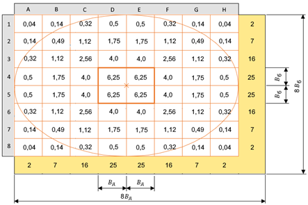
Figure. 1. Probability (in %) of projectiles hitting the cells of a rectangle described around the dispersion ellipse. The cell sizes are equal to the median deviations along the range B _d and along the front B _b. The yellow background indicates the total probability of a projectile hitting the corresponding band of the dispersion ellipse (i.e., the values ​​on the yellow background in each column A, B, etc. are equal to the sum of the numbers in all cells of this column, and the values ​​on the yellow background in each row 1, 2, etc. are equal to the sum of the numbers in all cells of this row).

In our case, as the likelihood function, we choose the probability value P with which the dispersion of shells can be exactly the same as it turned out to be as a result of this shelling. In this case, the value of the likelihood function P is determined from at least five partial likelihood functions for individual (“ control ”) areas of the dispersion ellipse:

P = min{ P _1; P_2 ; P_3 ; P_4 ; P_5 } (1)

where  P_k is the partial likelihood function for the k region of the dispersion ellipse as the probability that exactly as many shells will hit this region as actually hit ( k = 1 ... 5); in this case: - the first area ( k  = 1) is the small central square D4:E5; - the second area ( k  = 2) is the area outside the rectangle describing the ellipse; - the third area ( k  = 3) is a layer consisting of cells C3:F3, C6:F6, C4:C5 and F4:F5; - the fourth area ( k  = 4) is the large central square C3:F6; - the fifth area ( k  = 5) is a layer consisting of cells B2:G2, B7:G7, B3:B6 and G3:G6.

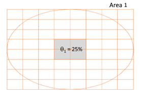
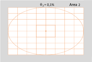
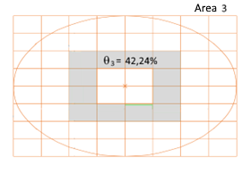
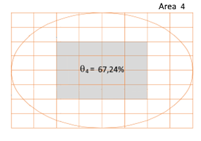
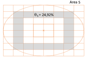Figure. 2. Theoretical probability of falling into different areas of the scattering ellipse, calculated by summing the values ​​in the corresponding cells from Fig. 1 (for region 2 it is conventionally taken to be 0.1% in order to avoid division by zero in formula (2)). 

Each of the probabilities  P _ k (where k  = 1...5) is determined from the table of the Pearson distribution function ( h ^2) [5, p. 140] with the number of degrees of freedom equal to 1 and the value of the argument [6, p. 628]:

h _ k ^2 = ( m _ k - n*t _ k )^2 / ( n*t _ k* (1 - t _ k )) (2)

where  m _ k is the number of projectiles (arrival points) that actually fell into the k region of the dispersion ellipse; n is the total number of shells in this sample (confirmed as arrival points); t_k - theoretical probability of getting into the k - th region of the dispersion ellipse (see Fig. 2): t_1 = 0.25;  t_2 = 0.001; t_3 = 0.4224; t_4 = 0.6724; t_5 = 0.2492. Criterion (2) characterizes the degree of deviation of the observed numbers from the theoretical ones n*t _ k . 

We will illustrate the described approach using the example of calculating the likelihood function and estimating the range of the shot point in one of the real examples. The total number of shells in this sample is 21. All of them are shown in Fig. 3a-3c in the form of a scatter diagram in the base coordinate system.

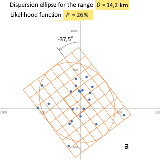
In Fig. 3a-3c, the scattering ellipses of projectiles without brake rings are superimposed on the arrival point diagram, constructed according to the median deviations B d and B b from the corresponding Firing Table for three different firing point ranges: 14.2, 16 and 18 km. The center of the ellipse is aligned with the center of point dispersion, the axes of the ellipse are tilted according to the known azimuth of the shot point (-37.5)°.

Figure 3. Scatter plot of projectile arrivals in the analyzed sample. Values ​​along the coordinate axes are in meters. The diagrams differ only in the dispersion ellipses, constructed according to the standard values ​​of the median deviations V d and V b for different values ​​of the range of the shot point: a - 14.2 km ( V d = 138 m, V b = 113 m), b - 16 km ( V d = 127 m, B b = 132 m), c – 18 km ( B d = 116 m, B b = 157 m). The inclination of the ellipse axes in all three diagrams is the same and corresponds to the azimuth of the shot point (-37.5)°.

For the dispersion ellipse corresponding to the shot point range of 14.2 km (Fig. 3 a), only 3 points fall into region 1, whereas theoretically there should be an average of n*t_1 =  21 * 0.25 = 5.25. Pearson criterion (2) in this case is equal to:

h_1 ^2 = (3 - 5.25)^2 / (5.25 * (1 - 0.25)) = 1.286 (3) 

According to the Pearson distribution function table, this value h ^2 = 1.286 corresponds to a probability of 0.26, i.e. P_1 = 0.26 = 26%. In other words, in approximately one case out of four, 3 out of 21 projectiles can hit the small central square of the dispersion ellipse. 

Somewhat more plausible at a range of 14.2 km is that twelve shells hit the large central square of the dispersion ellipse (area 4) instead of the theoretical  n*t_1 =  21  * 0.6724 = 14.12. Pearson criterion (2) in this case is equal to:

h_4 ^2 = (12 - 14.12)^2 / (14.12 * (1 - 0.06724)) = 0.972 (4)

and this value corresponds to a probability of 0.32, i.e. P_4 = 0.32 = 32%. 

The values ​​of the partial likelihood functions for all areas of the dispersion ellipse corresponding to a range of 14.2 km are as follows: P_1 = 26%, P_2 = 65%, P_3 = 97%, P_4 = 32%, P_5 = 91%. The smallest of these values ​​(26%) is the value of the final likelihood function, i.e. for a range of D = 14.2 km, the value of the likelihood function is 26 percent: P = 26%. 

In the case of a dispersion ellipse corresponding to a range of 16 km (Fig. 3 in the center), 4 points fall into the small central square (area 1), which is very close to the theoretical value of 5.25 and corresponds to the probability P_1 = 53%, and in the large the central square (area 4) hits 13 points, which corresponds to an even higher probability P_4 = 60%. In general, the final value of the likelihood function for the range D = 16 km is approximately twice as large as for 14.2 km, and is P = 53%. 

For a dispersion ellipse corresponding to a range of 18 km (Fig. 3 on the right), 5 points fall into the small central square, which practically coincides with the theoretical value of 5.25 and is therefore very plausible (probability P_1 = 90%). However, in the other two control regions of the ellipse, the partial likelihood functions are very small. Thus, 1 point falls outside the describing rectangle (area 2), (probability of such an event is P_2 = 0%), and only 2 points fall into area 5 instead of 5.23 (probability P_5 = 10%). Therefore, the value of the final likelihood function for a range of D = 18 km is very small and amounts to 0 percent: P = 0%.  

Similar calculations were performed for all values ​​of the firing point range in increments from the corresponding Shooting Table. The results of these calculations are shown in Fig. 4 (black dots connected by a thin line).

To eliminate the sensitivity of the results to the position of points on the boundaries between the cells of the scattering ellipse, two-stage averaging is used: 1) over range and 2) over azimuth.

Range averaging is performed over the five closest range values ​​from the Firing Table, i.e. calculate the range-averaged likelihood function P_avg . An example of a graph of the range-averaged likelihood function is shown in Fig. 4.

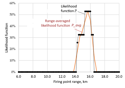Figure 4. Example of graphs of the likelihood function and its value
averaged over the range (azimuth of the shot point (-37.5)°). 

Averaging over azimuth is performed in the range of ±5° relative to the most probable azimuth value. For this purpose, for each range Di from the Firing Table, the values ​​calculated at seven different azimuths in the specified range are averaged.

Obtaining a likelihood function generalized over range and azimuth is illustrated in Fig. 5 (to simplify visual perception, this figure shows graphs of the range-averaged likelihood function for only three, and not for all seven azimuth values).

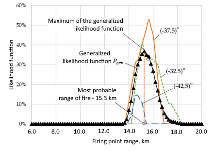
Figure 5. Illustration for the definition of the likelihood function generalized over range
and azimuth. Lines without markers show graphs of the range-averaged
likelihood function for specific values ​​of the azimuth of the shot point (labels next to the curves). The maximum of the generalized likelihood function corresponds to the most probable range of the shot point (in this example it is 15.3 km).

The maximum of the graph of the generalized likelihood function corresponds to the most probable range of the shot point (in the example shown in Fig. 5, the maximum of the generalized likelihood function is 38% and corresponds to the range of the shot point of 15.3 km).

The resulting generalized likelihood function was normalized relative to its maximum value in order to abstract from the numerical values ​​of the probability (what is important is not the absolute, but the relative values, i.e., how more or less plausible is one value of the shooting point range relative to another). As a result, we found the normalized likelihood function :

P _norm( D _ j ) = P _gen( D _ j ) / [ P _gen ]_ max    (5)

The correspondence between the generalized and normalized likelihood function is illustrated in Fig. 6. It is the normalized likelihood function that is proposed to be used to estimate the most probable range of the shot point.

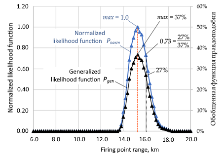
Rice. 6. Explanation of the definition of the normalized likelihood function

References

1. Appendix J. Crater analysis and reporting. https://www.globalsecurity.org/military/library/policy/army/fm/6-50/Appj.htm
2. Robert S. Yuill. The Standard Deviational Ellipse. An Updated Tool for Spatial Description. Geografiska Annaler. Series B, Human Geography, Vol. 53, No. 1 (1971), p. 28-39. http://www.jstor.org/stable/490885
3. Orlov A.R. Fundamentals of the functioning of multiple launch rocket system shells: Textbook. allowance. Tula: Tula Publishing House. state University, 2002. – 156 p.
4. Stolboshinsky A.P. Artillery course. Book 8. Probability theory. Scattering when shooting. M.: Military publishing house Min. Armed Forces of the USSR, 1949. – 282 p.
5. Bolshev L. N., Smirnov N. V. Tables of mathematical statistics. M.: Nauka, 1983. - 416 p.
6. Hald A. Mathematical statistics with technical applications. M.: Foreign Literature Publishing House, 1956. – 664 p.